


Forecasting Ford GoBike Demand
Sure looking at trends and extracting data might be useful as seen in this exploratory analysis I did but it sure would be much more useful to actually have some kind of model that did prediction around the data. Fortunately this data set comes with quite a few features that lend themselves to classification as well as time series analysis
Classification vs. Regression
For those newer to prediction and learning algorithms, classification is a set of machine learning techniques used to predict the label for an instance of data. Namely, the feature to predict is something discrete like the color of a car, whether a credit transaction is real or fraudulent, etc. where regression aims to predict the value of a continuous variable like a person's height, the length of a bike ride, etc.
Furthermore, we'll be working with supervised learning algorithms for this project. Supervised learning means creating some model that predicts an input-output pair based on input-output pairs that exist in the data. Essentially, the data contains the actual label of the instance that we're trying to classify so that we can actually compare our predicted value against it.
For classification in this project, we could try predicting the gender of the rider or whether the rider was a subscriber or customer. For regression, we'll be looking to predict the number of rides per day or even the length of a ride.
Anatomy of Building a Learning Model
Building a good learning model entails lots of steps which include, but are not limited to:
Choosing a learning technique
Training/Validation
Feature Engineering
Preventing Overfitting/Underfitting
At the code of every learning model is splitting the provided data into 3 sets: training, validation, and testing. The training data is used to build the model which is then validated against the holdout validation set of data to understand which model/parameters provide the best accuracy before taking the final model and running it on the test data. The importance of each of these cannot be overstated. We cannot simply train a model on all of the data since our model would be too specific to the set of data presented to us. Additionally a validation dataset is needed because evaluating the model and it's accuracy on a testing dataset (extracted from the whole dataset) without a validation dataset introduces bias into our model evaluation.
Without going into too much detail, feature engineering involves the adding/dropping/manipulating of features in the data to build the best model.
Lastly, we should be preventing overfitting and underfitting; overfitting being a model that is too specific to the training data and performs poorly on validation/test data and underfitting being a model that doesn't learn from the data enough and is too general and also performs poorly as a result. There are techniques for evaluating the strength of a model alongside the proper tradeoff between bias and variance but I won't jump into too much detail in this post.
Classifying Gender and User Type
When doing classification, I frequently find myself turning towards decision trees first before using more advanced techniques like SVM. Not only are decision trees easy to visualize and intuitively understand, they handle a mix of categorical and numerical data well and are relatively performant while being non-parametric. However, without pruning, they can be prone to overfitting and are sensitive to slight fluctuations in the data presented to the model in the data. Thankfully we can turn towards random forests to alleviate both these problems.
Decision trees are also prone to overfitting. Namely, this occurs when a learning model is modeled too specifically to the structure of the training data and performs poorly on the actual validation or test data. What this also means is that the learning algorithm can be pretty sensitive to the structure of the data. In general, classification algorithms can struggle against datasets that are severely unbalanced. What we mean by that is that for the target we're predicting, the label is predominantly of one class.
A classic example of this is in credit card fraud datasets. Clearly the vast majority of data points are perfectly valid transactions. However, a learning algorithm may very well just always predict that a transaction is valid since that might result in very high model accuracy. Clearly this provides a terrible false negative rate (transactions predicted to be valid when they are really fraud). To combat this, we should evaluate metrics like precision and recall or come up with better sampling strategies for the data to artificially create a balanced dataset.
As we discovered in the exploratory analysis of the Ford GoBike dataset, the vast majority of rides are taken by subscribers and a majority of the rides are taken by males. As a result, we have a similar situation albeit to a slightly less severe degree.
Two strategies to the problem above are to either downsample or upsample the majority or minority label, respectively. In downsampling, we randomly sample n pieces of data with the overrepresented label where n is equal to the number of pieces of data with the underrepresented data. The idea behind this is to effectively balance the dataset so the learning algorithm isn't incentivized to just "vote" on and, as as a result, classify as the majority label.
On the other hand, we can also oversample the minority label via a technique called SMOTE (Synthetic Minority Oversampling Technique). Again without going into too much detail, SMOTE works by finding the k-nearest neighbors for an instance of the minority class, taking the vector between it and a random neighbor and scaling it by some random factor between (0,1] to create a synthetic data point. This is then repeated until the desired ratio between the overrepresented and underrepresented labels is reached (for our case, we'll go with 1.0).
Finally to prepare the data for the decision tree classier, we want to encode the categorical variables like "Day of Week." Using the preprocessing library, we can use the LabelEncoder function to map each level of the categorical to a corresponding numerical variable for better consumption by learning algorithms. As for features, we'll use the following for now:
Duration
Start Hour
Day of Week
Age
User Type/Gender depending on the target variable
i.e. If predicting gender, add user type as a feature
Below we see the confusion matrices showing the predicted vs actual values for Gender. Strangely enough the balanced datasets actually result in worse performance, particularly for the downsampled dataset. The upsampled via SMOTE dataset has similar accuracy and recall but significantly worse precision.
Unbalanced
Now we can take a look at user type. To make sure that the decision tree wasn't classifying based on the majority class with the same ratio of it's appearance I found the majority to minority label ratio. As it turns out, 90.04% of users were subscribers so based on accuracy it at least appears that the decision tree is actually doing something non-trivial. Once again we see that predictive performance greatly suffers using via downsampling. The oversampled dataset has nearly identical accuracy, much worse precision and a nearly negligible improvement in recall. Once again, it seems that the unbalanced tree provides the best balance of results.
Unbalanced
It was not immediately clear to me what balancing the data would actually result in worse performance so I thought it was potentially the structure and localization of the data splits that just happened to have worse performance. I tried changing the random seed of the train_test_split function but to no avail.
In a last ditch effort, I swapped over to bagging by using Random Forests. Random Forests are an ensemble method that chorales a number of decision trees and then outputs either the mode of the decision tree outputs (classification) or the median (regression). While Random Forests can alleviate some of the overfitting issues presented by individual decision trees, they are also harder to understand and decipher. For the purpose of testing Random Forests here, I tried models built with 25, 50 and 100 decision trees. Unfortunately, I still saw very similar results with Random Forests although the upsampled Random Forest had a non-trivial improvement in recall (about 4%).
Unsatisfied and confused, I did a bit of reading to try and understand why this was occurring. From what I have learned and interpreted, my data isn't really quite as unbalanced as I thought. Upsampling, and balancing data, is significantly more effective when the minority target has an extremely low occurrence compared to the majority class (think <5%). From some readings, it seems that decision trees are also somewhat resilient to imbalance in data and the imbalance itself feeds information to the learning algorithm that can be used to infer about the classification. Lastly, it might just be that none of the features provide strong predictive value for the target. I'll seek to do some more feature engineering or evaluation of the importance of features in future blog posts but for now I'd like to jump into forecasting ride demand.
Forecasting Ride Demand
The most useful thing we could do with this data is provide some kind of forecasting for bike demand with a model given historical data. For data that both trends and has cyclic components, time series analysis and, more specifically, ARIMA comes into play for modeling.
ARIMA stands for AutoRegressive Integrated Moving Average and captures a spectrum of temporal characteristics for time series. Each component of this self-descriptive model has a corresponding parameter:
AR/p: Captures the lag in observations and other observations
I/d: The degree of differencing to make the data stationary
MA/q: Size of the moving average window in a model that uses the dependency between an observation and the residual error of a moving average window.
Without jumping too much into the complexities of each parameter, the goal here is to develop the best ARIMA model by optimizing the parameters to minimize RMSE (root mean squared error).
To approach creating an ARIMA model, we should first establish a baseline model and RMSE. To do this, we need to first split the data into training data and on which we will predict future ride volume. To do this, we can take the first n/2 days (where n is the total number of days that we have ride volume information for) to train on and predict the remaining n/2 days. For a baseline model, we can just create a model with a lag of 1. In essence, this just means that each day we will predict ride volume for the day to be equal to whatever the ride volume actually was on the immediately previous day.
To illustrate this, we'll look at the most popular station, Powell St BART Station.
Actual
In the first graph, above we split the data into the training (blue) and test (red). In the second graph we see that the predicted (yellow) is the same as the actual number of rides (green) albeit shifted by a lag of 1. This results in a model with RMSE = 43.12.
One important thing to know about ARIMA is that it assumes the time series is stationary. A stationary process is one in which the mean, variance and autocorrelation structure does not change over time. Clearly from the graph above, the time series appears non-stationary. The first thing we must do is transform the data into one which is. What we should expect to see is a time series without seasonality, constant variance and constant autocorrelation structure. Fortunately, we can difference the data and then test whether the resulting series is stationary via a statistical test, namely the Dickey-Fuller test.
One method of converting non-stationary data into stationary data is via differencing. In this technique, a differencing with degree 1 transforms the values:
(X1, X2, X3, X4,...Xn-1)
into
(X2-X1, X3-X2, X4-X3,...Xn-Xn-1)
If differencing with degree 1 still does not result in a stationary series, a higher order can be considered. However this makes the analysis more complicated. The below graph shows the data with degree 1 differencing.
ADF (Augmented Dickey-Fuller) Statistic: -6.744385
p-value: 0.000000
Critical Values:
1%: -3.449
5%: -2.870
10%: -2.571
Here, the ADF statistic is smaller than the 1% critical value statistic meaning we can reject the null hypothesis which in returns means the data is stationary.
Lastly we can review the ACF and PACF plots to guide some good values for ARIMA parameters. ACF plots tell us the amount of lag after which autocorrelation becomes insignificant. From our plot below it seems that autocorrelation is significant for a decent number of lags despite dropping exponentially. However, looking at the PACF plot confirms that the autocorrelation at lags 2 and above are due to the propagation of autocorrelation at lag 1. Unfortunately, the ACF/PACF plots show that there is not insignificant lag so we can assume that the best parameters will not be a value of 0 for each parameter. Knowing the structure of the data and the cyclical structure of bike demand on a weekly basis, a good starting value for the p parameter may be something around 7.

In order to find the best ARIMA model, we'll implement grid search for the parameter tuning. In short, grid search is a method used to explore every unique combination of values for parameters in order to find the set that results in the best model. The computational complexity of the ARIMA model becomes significantly more heavy as the p parameter increases in magnitude so I performed grid search on the following ranges:
p: [0,8)
d: [0,3)
q: [0,2)
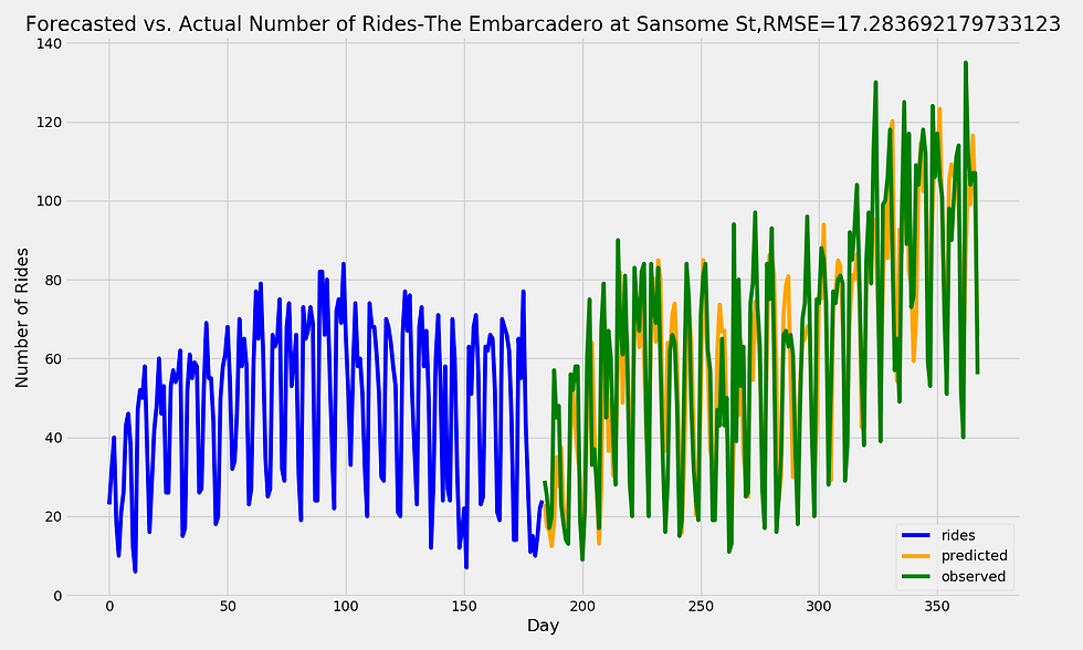
After evaluating each model for Powell St BART Station using each unique combination of parameters above, the model with the lowest RMSE of 26.478 uses p=7, d=1, q=1. The prediction from the model is plotted below:

Clearly there are a few points where ARIMA either over-predicted or under-predicted the ride demand for the day. However, what is extremely impressive is that the cyclical nature of the demand is caught without lag and the increasing trend in demand is captured as well.
I ran a grid search for optimal ARIMA parameters for each of the stations below and also plotted out the prediction from the model:


Closing Thoughts
Something I need to do more of is actually doing machine learning/prediction instead of just exploratory data analysis. This is my first real foray into time series analysis and forecasting so it was highly educational and interesting. Of course there is still a ton more to learn including all of the theory behind it (the kind of stuff backing SVMs, Markov chains, logistic regression, etc that I loved studying). I think I'll aim to make my next project something classification related!
As always, shoot me a message with suggestions or comments. You can find the code behind all of this here: Ford GoBike Prediction.
Comments